GS interview

Author: Chen Zhiyuan §

Date: 2024-03-10 §

GSinterview Project §

Abstract §

This interview project focuses on predicting rebar demand using a combination of time-series forecasting (Prophet), machine learning regression (XGBoost), and deep learning (LSTM). Given the volatile nature of rebar demand influenced by economic and construction activity, we leverage multiple models to capture both short-term fluctuations and long-term trends. The models are combined using an ensemble weighted averaging approach optimized via Bayesian Optimization. My results demonstrate that XGBoost and Prophet contribute the most to the final forecast, while LSTM provides minimal impact due to its lower predictive accuracy.

Data Cleaning and Manipulaiton §

1. Data Merging §

The dataset consisted of multiple sources, including rebar demand, rebar price, cement demand, real estate growth, and infrastructure growth. To create a unified dataset:

• Data was merged on a weekly time index using the “date_demand” column.

• Different datasets were joined using an outer join strategy to avoid unintentional data loss.

• Missing values after merging were handled appropriately (detailed below).

2. Handling Missing Values §

• Rebar Price: Missing weekly values were filled using the mean rebar price for the corresponding month.

• Cement Demand: Missing entries were interpolated based on previous and next available values.

• Real Estate & Infrastructure Growth: Forward fill and backward fill techniques were applied to maintain time consistency.

• Final Imputation: For any remaining missing values, I used linear interpolation where necessary.

3. Feature Engineering §

To enhance model performance, I engineered additional features:

• Lagged Features: Created for rebar_demand and cement_demand using best_lags = [1, 2, 3, 4, 12] to capture short-term and longer-term patterns.

• Temporal Encoding:

  • Applied sin-cos encoding to transform cyclical variables such as month and week_of_month to better represent seasonality.

  • Created month_sin, month_cos, and week_sin as new features.

• Normalization: Applied MinMaxScaler for XGBoost and LSTM models to standardize data ranges.

4. Overview §

• Number of Samples: 218 total rows after merging.

• Final Features Used:

  • Economic indicators: cement_demand, real_estate_growth, infra_growth.

  • Engineered features: rebar_demand_lag_X, cement_demand_lag_X (for X in best_lags).

  • Time-based encodings: month_sin, month_cos, week_sin.

• Target Variable: rebar_demand.

EDA & Time-Series Modeling §

1. Trends of Rebar Demand and Related Variabl §

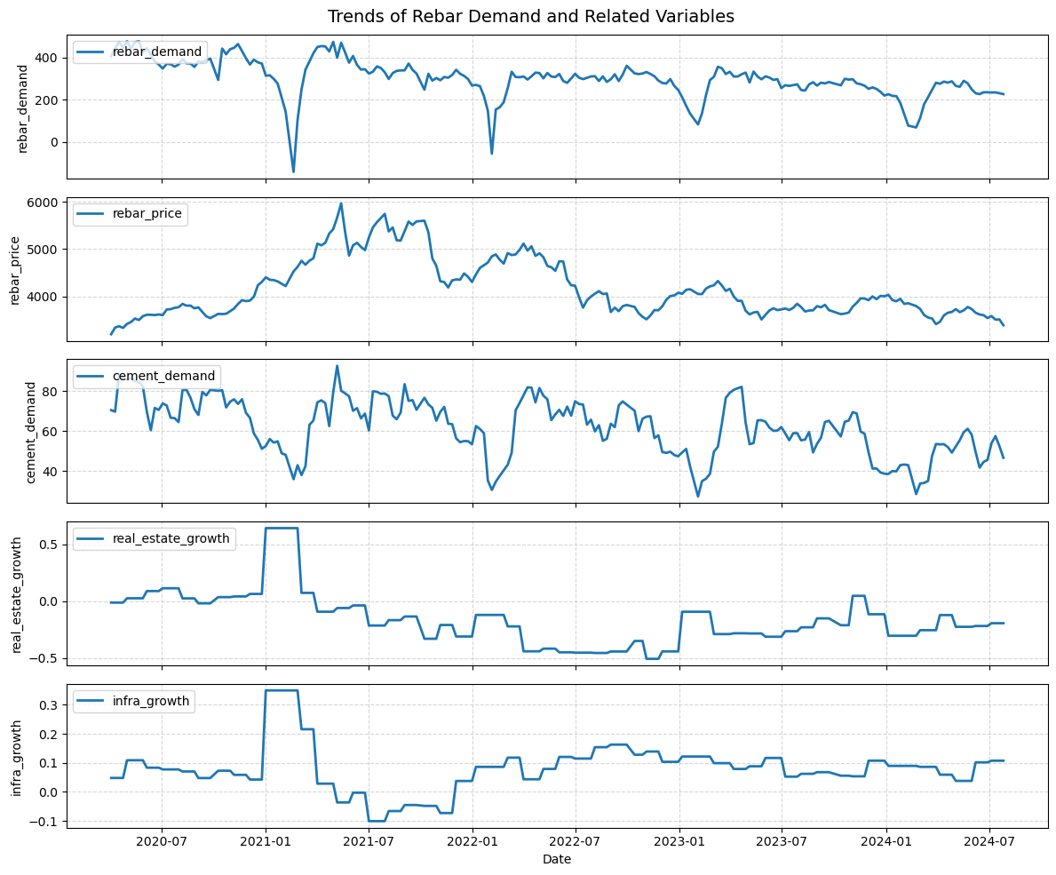
To understand the key drivers of rebar demand, I visualized its relationship with other economic indicators:

• Rebar Demand: Displays fluctuations over time, with clear seasonal patterns and occasional sharp drops.

• Rebar Price: Shows an upward trend, peaking around 2021 before stabilizing.

• Cement Demand: Exhibits high volatility, with peaks and troughs that often align with rebar demand.

• Real Estate & Infrastructure Growth: These variables show moderate fluctuations, suggesting possible influence on rebar demand.

2. Correlation Between Variables §

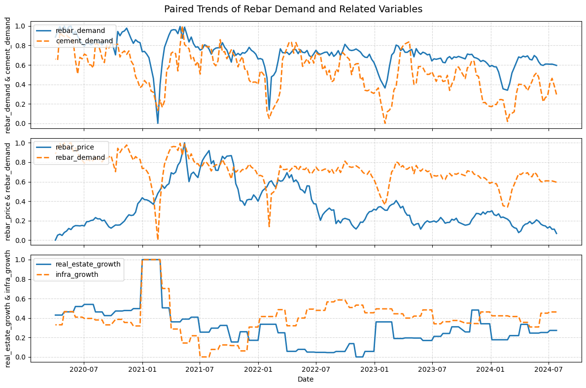
• The relationship between cement demand and rebar demand appears strong, indicating that construction activity drives demand for both materials.

• Rebar price and demand show a negative correlation, meaning that as prices rise, demand tends to decrease.

• Infrastructure growth and real estate growth show some correlation with rebar demand, but the relationship is less direct.

3. Seasonality and Monthly Patterns §

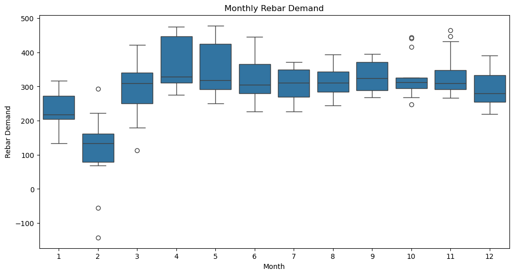• A box plot of monthly demand reveals that certain months (April-July) experience higher demand, whereas February tends to have lower demand.

• This suggests a seasonal component, likely influenced by weather conditions and construction cycles.

4. Time-Series Characteristics §

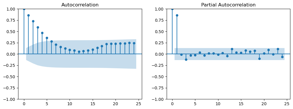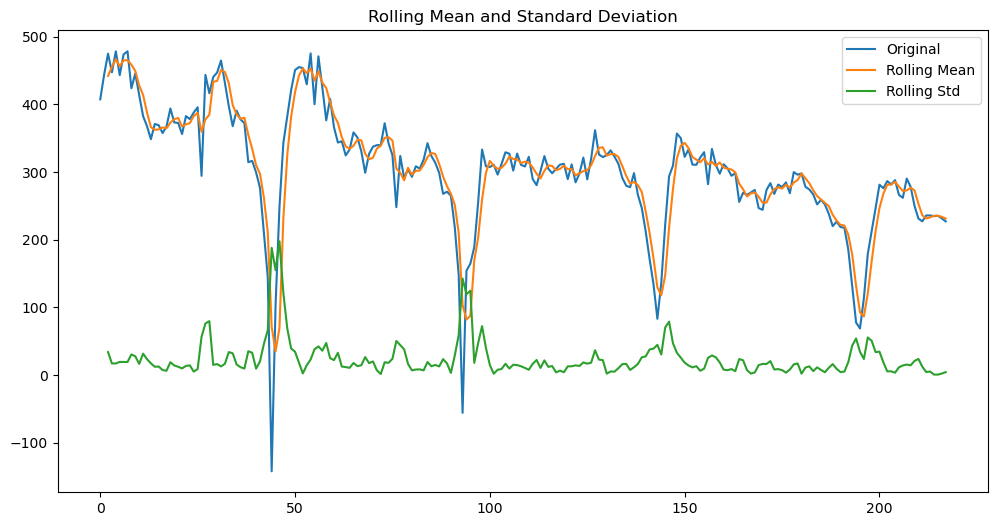
Autocorrelation and Partial Autocorrelation Plots suggest that past demand values significantly influence future values, confirming the necessity of lag features in modeling. Rolling Mean and Standard Deviation plots indicate that the series is not strictly stationary, requiring transformations for time-series forecasting. 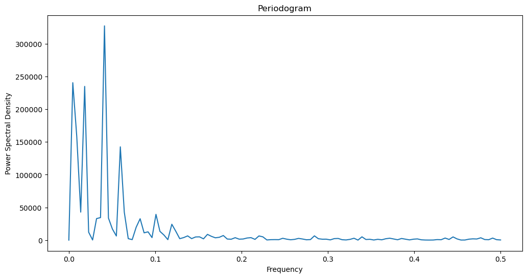Periodogram Analysis reveals strong frequency components, reinforcing the presence of seasonal patterns.

5. Lag Analysis §

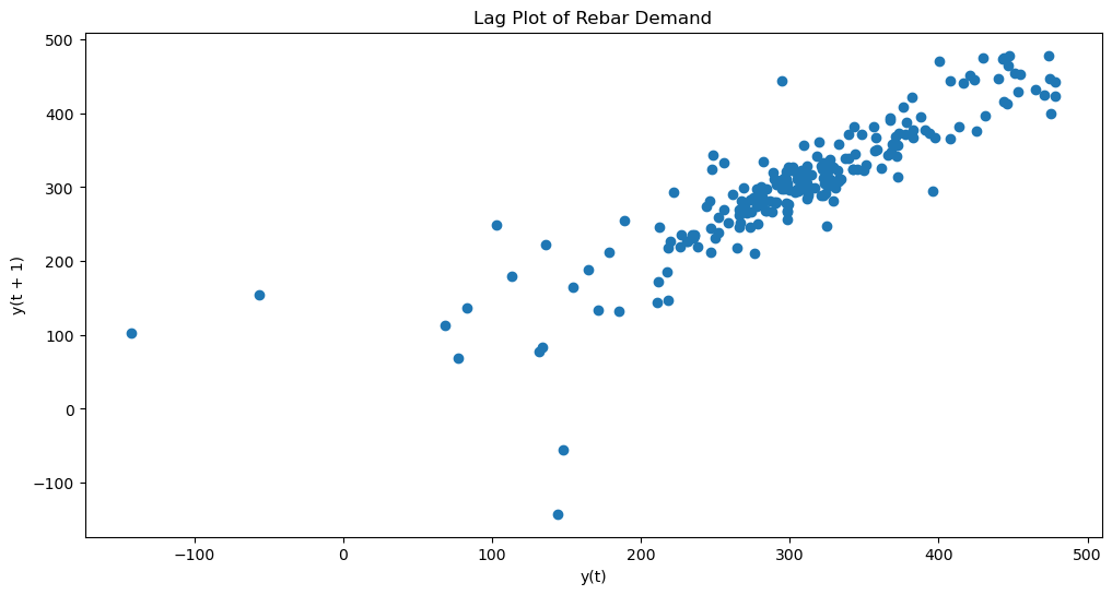
A lag plot of rebar demand shows a strong linear relationship between demand at time t and t+1, further supporting the inclusion of lagged features.

Modeling §

Problem Formulation: §

The objective of this study is to forecast rebar demand using historical data and key economic indicators. Given the time-dependent nature of the data, we implemented a combination of:

• Time-Series Forecasting (Prophet): Ability to model seasonality, trends, and external factors with high interpretability.

• Machine Learning Regression (XGBoost with Bayesian Optimization) Strength in capturing complex non-linear relationships from engineered features. • Deep Learning (LSTM) Ability to learn long-term dependencies in sequential data without manual feature engineering. • Ensemble Learning (Weighted Averaging with Bayesian Optimization) Allows to leverage their strengths, balancing interpretability, robustness, and predictive accuracy.

Feature Engineering: §

• Lagged Features: Created past demand values as predictors, using lags [1, 2, 3, 4, 12].

• Rolling Statistics: Included rolling mean and rolling standard deviation to capture recent trends.

• Seasonal Indicators: Introduced cyclic features (month_sin, month_cos, week_sin) to capture monthly and weekly trends.

• Macroeconomic Indicators: Incorporated cement demand, real estate growth, and infrastructure growth to account for broader market effects.

Model Selection & Training §

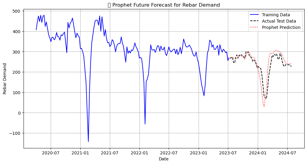
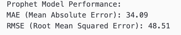
a. Prophet(Time-Series Model) • Automatically detects trends and seasonality in data.

• Used additive seasonality and a weekly granularity (freq=“W”).

• Generated future forecasts and aligned with actual test data.

---

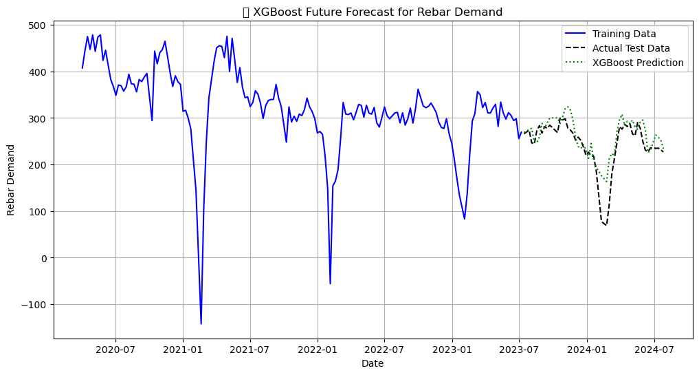
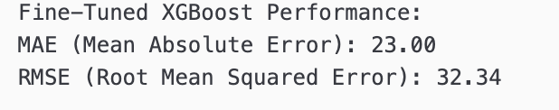
b. XGBoost (Gradient Boosting Machine)

• Trained using engineered features.

• Fine-tuned using Bayesian Optimization for hyperparameter selection.

• Outperformed baseline models by capturing complex feature interactions.

---

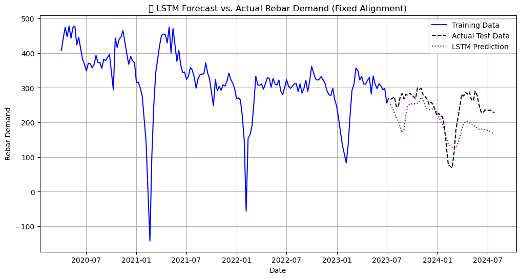
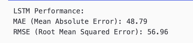
C. LSTM (Deep Learning for Time-Series) • Designed a two-layer LSTM with ReLU and “Tanh” activation and dropout layers.

• Used sequence_length = 12, meaning the model learns patterns from the past 12 weeks.

• Predictions were rescaled back to the original demand range.

---

Ensemble Model (Optimized Weights) §

Instead of relying on a single model, we combined all three models using Weighted Averaging:

• Weight Optimization: Used Bayesian Optimization to find the best weight combination

Optimized Weights → Prophet: 0.420+ XGBoost: 0.333+ LSTM: 0.247

**Optimized Ensemble RMSE: 21.08 **

Conclusion §

• This project demonstrates that an ensemble approach combining Prophet and XGBoost provides the best rebar demand forecast. LSTM’s performance was weaker, possibly due to its sensitivity to small datasets or suboptimal architecture. The optimized ensemble model achieved an RMSE of 21.08, significantly improving upon individual models.

• Feature Expansion:

  • Include additional macroeconomic indicators (e.g., GDP, steel demand, government infrastructure spending).

  • Incorporate weather conditions, which may affect construction activity.